Demo 2: HKR Classifier on toy dataset
In this demo notebook we will show how to build a robust classifier
based on the regularized version of the Kantorovitch-Rubinstein duality.
We will perform this on the two moons synthetic dataset.
from datetime import datetime
import os
import numpy as np
import math

from sklearn.datasets import make_moons, make_circles  # the synthetic dataset

import matplotlib.pyplot as plt
import seaborn as sns

from wasserstein_utils.otp_utils import otp_generator  # keras generator of the synthetic dataset

# in order to build our classifier we will use element from tensorflow along with
# layers from deel-lip
import tensorflow as tf
from tensorflow.keras import backend as K
from tensorflow.keras.layers import ReLU, Input
from tensorflow.keras.optimizers import Adam
from tensorflow.keras.callbacks import ReduceLROnPlateau
from tensorflow.keras.metrics import binary_accuracy

from deel.lip.model import Model  # use of deel.lip is not mandatory but offers the vanilla_export feature
from deel.lip.layers import SpectralConv2D, SpectralDense, FrobeniusDense
from deel.lip.activations import MaxMin, GroupSort, FullSort, GroupSort2
from deel.lip.utils import load_model  # wrapper that avoid manually specifying custom_objects field
from deel.lip.losses import HKR_loss, KR_loss, hinge_margin_loss  # custom losses for HKR robust classif
from deel.lip.normalizers import DEFAULT_NITER_BJORCK, DEFAULT_NITER_SPECTRAL

from model_samples.model_samples import get_lipMLP  # helper to quickly build an HKR classifier
Parameters
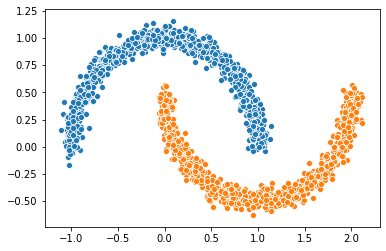
Let’s first construct our two moons dataset
circle_or_moons = 1  # 0 for circle , 1 for moons
n_samples=5000  # number of sample in the dataset
noise=0.05  # amount of noise to add in the data. Tested with 0.14 for circles 0.05 for two moons
factor=0.4  # scale factor between the inner and the outer circle
if circle_or_moons == 0:
    X,Y=make_circles(n_samples=n_samples,noise=noise,factor=factor)
else:
    X,Y=make_moons(n_samples=n_samples,noise=noise)

# When working with the HKR-classifier, using labels {-1, 1} instead of {0, 1} is advised.
# This will be explained further on
Y[Y==1]=-1
Y[Y==0]=1
X1=X[Y==1]
X2=X[Y==-1]
sns.scatterplot(X1[:1000,0],X1[:1000,1])
sns.scatterplot(X2[:1000,0],X2[:1000,1])
<matplotlib.axes._subplots.AxesSubplot at 0x2c40c220208>
Relation with optimal transport
In this setup we can solve the optimal transport problem between the
distribution of X[Y==1] and X[Y==-1]. This usually require to
match each element of the first distribution with an element of the
second distribution such that this minimize a global cost. In our setup
this cost is the $ l_1 $ distance, which will allow us to make use of
the KR dual formulation. The overall cost is then the \(W_1\)
distance.
However the \(W_1\) distance is known to be untractable in general.
KR dual formulation
In our setup, the KR dual formulation is stated as following:
This state the problem as an optimization problem over the 1-lipschitz functions. Therefore k-Lipschitz networks allows us to solve this maximization problem.
Hinge-KR classification
When dealing with \(W_1\) one may note that many functions maximize the maximization problem described above. Also we want this function to be meaningfull in terms of classification. To do so, we want f to be centered in 0, which can be done without altering the inital problem. By doing so we can use the obtained function for binary classification, by looking at the sign of \(f\).
In order to enforce this, we will add a Hinge term to the loss. It has been shown that this new problem is still a optimal transport problem and that this problem admit a meaningfull optimal solution.
HKR-Classifier
Now we will show how to build a binary classifier based on the regularized version of the KR dual problem.
In order to ensure the 1-Lipschitz constraint deel-lip uses spectral
normalization. These layers also can also use Bjork orthonormalization
to ensure that the gradient of the layer is 1 almost everywhere.
Experiment shows that the optimal solution lie in this sub-class of
functions.
batch_size=256
steps_per_epoch=40480
epoch=10
hidden_layers_size = [256,128,64]  # stucture of the network
niter_spectral = DEFAULT_NITER_SPECTRAL
niter_bjorck = DEFAULT_NITER_BJORCK
activation = FullSort  # other lipschitz activation are ReLU, MaxMin, GroupSort2, GroupSort
min_margin= 0.29  # minimum margin to enforce between the values of f for each class
# build data generator
gen=otp_generator(batch_size,X,Y)
Build lipschitz Model
Let’s build our model now.
K.clear_session()
wass=get_lipMLP(
    (2,),
    hidden_layers_size = hidden_layers_size,
    activation=activation,
    nb_classes = 1,
    kCoefLip=1.0,
    niter_spectral = niter_spectral,
    niter_bjorck = niter_bjorck
)
## please note that calling the previous helper function has the exact
## same effect as the following code:
# inputs = Input((2,))
# x = SpectralDense(256, activation=FullSort(),
#                   niter_spectral=niter_spectral,
#                   niter_bjorck=niter_bjorck)(inputs)
# x = SpectralDense(128, activation=FullSort(),
#                   niter_spectral=niter_spectral,
#                   niter_bjorck=niter_bjorck)(x)
# x = SpectralDense(64, activation=FullSort(),
#                   niter_spectral=niter_spectral,
#                   niter_bjorck=niter_bjorck)(x)
# y = FrobeniusDense(1, activation=None)(x)
# wass = Model(inputs=inputs, outputs=y)
wass.summary()
256
128
64
Model: "model"
_________________________________________________________________
Layer (type)                 Output Shape              Param #
=================================================================
input_1 (InputLayer)         [(None, 2)]               0
_________________________________________________________________
flatten (Flatten)            (None, 2)                 0
_________________________________________________________________
spectral_dense (SpectralDens (None, 256)               1025
_________________________________________________________________
full_sort (FullSort)         (None, 256)               0
_________________________________________________________________
spectral_dense_1 (SpectralDe (None, 128)               33025
_________________________________________________________________
full_sort_1 (FullSort)       (None, 128)               0
_________________________________________________________________
spectral_dense_2 (SpectralDe (None, 64)                8321
_________________________________________________________________
full_sort_2 (FullSort)       (None, 64)                0
_________________________________________________________________
frobenius_dense (FrobeniusDe (None, 1)                 65
=================================================================
Total params: 42,436
Trainable params: 41,985
Non-trainable params: 451
_________________________________________________________________
As we can see the network has a gradient equal to 1 almost everywhere as all the layers respect this property.
It is good to note that the last layer is a FrobeniusDense this is
because, when we have a single output, it become equivalent to normalize
the frobenius norm and the spectral norm (as we only have a single
singular value)
optimizer = Adam(lr=0.01)
# as the output of our classifier is in the real range [-1, 1], binary accuracy must be redefined
def HKR_binary_accuracy(y_true, y_pred):
    S_true= tf.dtypes.cast(tf.greater_equal(y_true[:,0], 0),dtype=tf.float32)
    S_pred= tf.dtypes.cast(tf.greater_equal(y_pred[:,0], 0),dtype=tf.float32)
    return binary_accuracy(S_true,S_pred)
wass.compile(
    loss=HKR_loss(alpha=10,min_margin=min_margin),  # HKR stands for the hinge regularized KR loss
    metrics=[
        KR_loss((-1,1)),  # shows the KR term of the loss
        hinge_margin_loss(min_margin=min_margin),  # shows the hinge term of the loss
        HKR_binary_accuracy  # shows the classification accuracy
    ],
    optimizer=optimizer
)
Learn classification on toy dataset
Now we are ready to learn the classification task on the two moons dataset.
wass.fit_generator(
    gen,
    steps_per_epoch=steps_per_epoch // batch_size,
    epochs=epoch,
    verbose=1
)
WARNING:tensorflow:From <ipython-input-11-258ce98fe6fe>:5: Model.fit_generator (from tensorflow.python.keras.engine.training) is deprecated and will be removed in a future version.
Instructions for updating:
Please use Model.fit, which supports generators.
WARNING:tensorflow:sample_weight modes were coerced from
  ...
    to
  ['...']
Train for 158 steps
Epoch 1/10
158/158 [==============================] - 5s 30ms/step - loss: -0.3610 - KR_loss_fct: -0.9315 - hinge_margin_fct: 0.0571 - HKR_binary_accuracy: 0.9176 4s - loss: 0.1094 - KR_loss_fct: -0.8685 - hinge_marg
Epoch 2/10
158/158 [==============================] - 2s 15ms/step - loss: -0.8084 - KR_loss_fct: -0.9796 - hinge_margin_fct: 0.0171 - HKR_binary_accuracy: 0.9890
Epoch 3/10
158/158 [==============================] - 2s 15ms/step - loss: -0.8202 - KR_loss_fct: -0.9858 - hinge_margin_fct: 0.0166 - HKR_binary_accuracy: 0.9895
Epoch 4/10
158/158 [==============================] - 2s 15ms/step - loss: -0.8313 - KR_loss_fct: -0.9949 - hinge_margin_fct: 0.0164 - HKR_binary_accuracy: 0.9894
Epoch 5/10
158/158 [==============================] - 3s 17ms/step - loss: -0.8239 - KR_loss_fct: -0.9818 - hinge_margin_fct: 0.0158 - HKR_binary_accuracy: 0.9903
Epoch 6/10
158/158 [==============================] - 3s 18ms/step - loss: -0.8229 - KR_loss_fct: -0.9896 - hinge_margin_fct: 0.0167 - HKR_binary_accuracy: 0.9891
Epoch 7/10
158/158 [==============================] - 3s 19ms/step - loss: -0.8361 - KR_loss_fct: -0.9911 - hinge_margin_fct: 0.0155 - HKR_binary_accuracy: 0.9908
Epoch 8/10
158/158 [==============================] - 3s 19ms/step - loss: -0.8333 - KR_loss_fct: -0.9941 - hinge_margin_fct: 0.0161 - HKR_binary_accuracy: 0.9899
Epoch 9/10
158/158 [==============================] - 3s 19ms/step - loss: -0.8315 - KR_loss_fct: -0.9945 - hinge_margin_fct: 0.0163 - HKR_binary_accuracy: 0.9895
Epoch 10/10
158/158 [==============================] - 3s 20ms/step - loss: -0.8438 - KR_loss_fct: -0.9913 - hinge_margin_fct: 0.0147 - HKR_binary_accuracy: 0.9925
<tensorflow.python.keras.callbacks.History at 0x2c40d92c388>
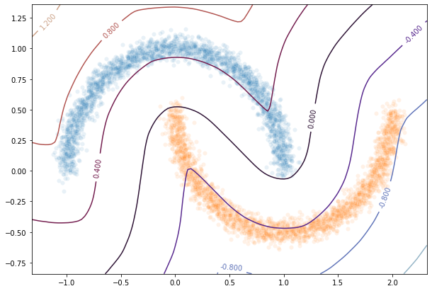
Plot output countour line
As we can see the classifier get a pretty good accuracy. Let’s now take a look at the learnt function. As we are in the 2D space, we can draw a countour plot to visualize f.
import matplotlib.pyplot as plt
from mpl_toolkits.mplot3d import Axes3D
from matplotlib import cm
from matplotlib.ticker import LinearLocator, FormatStrFormatter
batch_size=1024

x = np.linspace(X[:,0].min()-0.2, X[:,0].max()+0.2, 120)
y = np.linspace(X[:,1].min()-0.2, X[:,1].max()+0.2,120)
xx, yy = np.meshgrid(x, y, sparse=False)
X_pred=np.stack((xx.ravel(),yy.ravel()),axis=1)
# make predictions of f
pred=wass.predict(X_pred)

Y_pred=pred
Y_pred=Y_pred.reshape(x.shape[0],y.shape[0])
#plot the results
fig = plt.figure(figsize=(10,7))
ax1 = fig.add_subplot(111)

sns.scatterplot(X[Y==1,0],X[Y==1,1],alpha=0.1,ax=ax1)
sns.scatterplot(X[Y==-1,0],X[Y==-1,1],alpha=0.1,ax=ax1)
cset =ax1.contour(xx,yy,Y_pred,cmap='twilight')
ax1.clabel(cset, inline=1, fontsize=10)
<a list of 7 text.Text objects>

Transfer network to a classical MLP and compare outputs
As we saw, our networks use custom layers in order to constrain
training. However during inference layers behave exactly as regular
Dense or Conv2d layers. Deel-lip has a functionnality to export
a model to it’s vanilla keras equivalent. Making it more convenient for
inference.
from deel.lip.model import vanillaModel
## this is equivalent to test2 = wass.vanilla_export()
test2 = vanillaModel(wass)
test2.summary()
tensor input shape (None, 2)
tensor input shape (None, 2)
tensor input shape (None, 2)
tensor input shape (None, 256)
256
tensor input shape (None, 256)
tensor input shape (None, 128)
128
tensor input shape (None, 128)
tensor input shape (None, 64)
64
tensor input shape (None, 64)
Model: "model_1"
_________________________________________________________________
Layer (type)                 Output Shape              Param #
=================================================================
input_2 (InputLayer)         [(None, 2)]               0
_________________________________________________________________
flatten (Flatten)            (None, 2)                 0
_________________________________________________________________
spectral_dense (Dense)       (None, 256)               768
_________________________________________________________________
full_sort (FullSort)         (None, 256)               0
_________________________________________________________________
spectral_dense_1 (Dense)     (None, 128)               32896
_________________________________________________________________
full_sort_1 (FullSort)       (None, 128)               0
_________________________________________________________________
spectral_dense_2 (Dense)     (None, 64)                8256
_________________________________________________________________
full_sort_2 (FullSort)       (None, 64)                0
_________________________________________________________________
frobenius_dense (Dense)      (None, 1)                 65
=================================================================
Total params: 41,985
Trainable params: 41,985
Non-trainable params: 0
_________________________________________________________________
pred_test=test2.predict(X_pred)
Y_pred=pred_test
Y_pred=Y_pred.reshape(x.shape[0],y.shape[0])
fig = plt.figure(figsize=(10,7))
ax1 = fig.add_subplot(111)
#ax2 = fig.add_subplot(312)
#ax3 = fig.add_subplot(313)
sns.scatterplot(X[Y==1,0],X[Y==1,1],alpha=0.1,ax=ax1)
sns.scatterplot(X[Y==-1,0],X[Y==-1,1],alpha=0.1,ax=ax1)
cset =ax1.contour(xx,yy,Y_pred,cmap='twilight')
ax1.clabel(cset, inline=1, fontsize=10)
<a list of 7 text.Text objects>