Demo 1: Wasserstein distance estimation on toy example
In this notebook we will see how to estimate the wasserstein distance with a Neural net by using the Kantorovich-Rubinestein dual representation.
from datetime import datetime
import os
import numpy as np
import math

import matplotlib.pyplot as plt

from tensorflow.keras import backend as K
from tensorflow.keras.layers import Input, Flatten, ReLU
from tensorflow.keras.optimizers import Adam

from deel.lip.layers import SpectralConv2D, SpectralDense, FrobeniusDense
from deel.lip.activations import MaxMin, GroupSort, FullSort
from deel.lip.utils import load_model
from deel.lip.losses import KR_loss
from deel.lip.model import Model

from model_samples.model_samples import get_lipMLP
Parameters input images
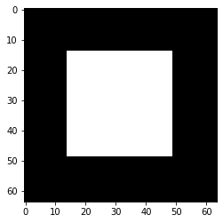
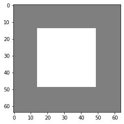
The synthetic dataset will be composed image with black or white squares allowing us to check if the computed wasserstein distance is correct.
img_size = 64
frac_value = 0.3  # proportion of the center square
Generate images
def generate_toy_images(shape,frac=0,v=1):
    """
    function that generate a single image.

    Args:
        shape: shape of the output image
        frac: proportion of the center square
        value: value assigned to the center square
    """
    img = np.zeros(shape)
    if frac==0:
        return img
    frac=frac**0.5
    #print(frac)
    l=int(shape[0]*frac)
    ldec=(shape[0]-l)//2
    #print(l)
    w=int(shape[1]*frac)
    wdec=(shape[1]-w)//2
    img[ldec:ldec+l,wdec:wdec+w,:]=v
    return img


def binary_generator(batch_size,shape,frac=0):
    """
    generate a batch with half of black images, hald of images with a white square.
    """
    batch_x = np.zeros(((batch_size,)+(shape)), dtype=np.float16)
    batch_y=np.zeros((batch_size,1), dtype=np.float16)
    batch_x[batch_size//2:,]=generate_toy_images(shape,frac=frac,v=1)
    batch_y[batch_size//2:]=1
    while True:
        yield  batch_x, batch_y


def ternary_generator(batch_size,shape,frac=0):
    """
    Same as binary generator, but images can have a white square of value 1, or value -1
    """
    batch_x = np.zeros(((batch_size,)+(shape)), dtype=np.float16)
    batch_y=np.zeros((batch_size,1), dtype=np.float16)
    batch_x[3*batch_size//4:,]=generate_toy_images(shape,frac=frac,v=1)
    batch_x[batch_size//2:3*batch_size//4,]=generate_toy_images(shape,frac=frac,v=-1)
    batch_y[batch_size//2:]=1
    #indexes_shuffle = np.arange(batch_size)
    while True:
        #np.random.shuffle(indexes_shuffle)
        #yield  batch_x[indexes_shuffle,], batch_y[indexes_shuffle,]
        yield  batch_x, batch_y
def display_img(img):
    """
    Display an image
    """
    if img.shape[-1] == 1:
        img = np.tile(img,(3,))
    fig, ax = plt.subplots()

    imgplot = ax.imshow((img*255).astype(np.uint))
Now let’s take a look at the generated batches
test=binary_generator(2,(img_size,img_size,1),frac=frac_value)
imgs, y=next(test)

display_img(imgs[0])
display_img(imgs[1])
print("Norm L2 "+str(np.linalg.norm(imgs[1])))
print("Norm L2(count pixels) "+str(math.sqrt(np.size(imgs[1][imgs[1]==1]))))
Norm L2 35.0
Norm L2(count pixels) 35.0
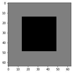
test=ternary_generator(4,(img_size,img_size,1),frac=frac_value)
imgs, y=next(test)

for i in range(4):
    display_img(0.5*(imgs[i]+1.0)) # we ensure that there is no negative value wehn displaying images

print("Norm L2(imgs[2]-imgs[0])"+str(np.linalg.norm(imgs[2]-imgs[0])))
print("Norm L2(imgs[2]) "+str(np.linalg.norm(imgs[2])))
print("Norm L2(count pixels) "+str(math.sqrt(np.size(imgs[2][imgs[2]==-1]))))
Norm L2(imgs[2]-imgs[0])35.0
Norm L2(imgs[2]) 35.0
Norm L2(count pixels) 35.0

Expe parameters
Now we know the wasserstein distance between the black image and the images with a square on it. For both binary generator and ternary generator this distance is 35.
We will then compute this distance using a neural network.
KR dual formulation
In our setup, the KR dual formulation is stated as following:
This state the problem as an optimization problem over the 1-lipschitz functions. Therefore k-Lipschitz networks allows us to solve this maximization problem.
[1] C. Anil, J. Lucas, et R. Grosse, « Sorting out Lipschitz function approximation », arXiv:1811.05381 [cs, stat], nov. 2018.
batch_size=64
epochs=5
steps_per_epoch=6400
generator = ternary_generator   #binary_generator, ternary_generator
activation = FullSort #ReLU, MaxMin, GroupSort
Build lipschitz Model
K.clear_session()
wass=get_lipMLP((img_size,img_size,1), hidden_layers_size = [128,64,32] ,activation=activation, nb_classes = 1,kCoefLip=1.0)
## please note that the previous helper function has the same behavior as the following code:
# inputs = Input((img_size, img_size, 1))
# x = SpectralDense(128, activation=FullSort())(inputs)
# x = SpectralDense(64, activation=FullSort())(x)
# x = SpectralDense(32, activation=FullSort())(x)
# y = FrobeniusDense(1, activation=None)(x)
# wass = Model(inputs=inputs, outputs=y)
wass.summary()
128
64
32
Model: "model"
_________________________________________________________________
Layer (type)                 Output Shape              Param #
=================================================================
input_1 (InputLayer)         [(None, 64, 64, 1)]       0
_________________________________________________________________
flatten (Flatten)            (None, 4096)              0
_________________________________________________________________
spectral_dense (SpectralDens (None, 128)               524545
_________________________________________________________________
full_sort (FullSort)         (None, 128)               0
_________________________________________________________________
spectral_dense_1 (SpectralDe (None, 64)                8321
_________________________________________________________________
full_sort_1 (FullSort)       (None, 64)                0
_________________________________________________________________
spectral_dense_2 (SpectralDe (None, 32)                2113
_________________________________________________________________
full_sort_2 (FullSort)       (None, 32)                0
_________________________________________________________________
frobenius_dense (FrobeniusDe (None, 1)                 33
=================================================================
Total params: 535,012
Trainable params: 534,785
Non-trainable params: 227
_________________________________________________________________
optimizer = Adam(lr=0.01)
wass.compile(loss=KR_loss(), optimizer=optimizer, metrics=[KR_loss()])
Learn on toy dataset
wass.fit_generator( generator(batch_size,(img_size,img_size,1),frac=frac_value),
                steps_per_epoch=steps_per_epoch// batch_size,
                epochs=epochs,verbose=1)
WARNING:tensorflow:From <ipython-input-12-b25f21272064>:3: Model.fit_generator (from tensorflow.python.keras.engine.training) is deprecated and will be removed in a future version.
Instructions for updating:
Please use Model.fit, which supports generators.
WARNING:tensorflow:sample_weight modes were coerced from
  ...
    to
  ['...']
Train for 100 steps
Epoch 1/5
100/100 [==============================] - 17s 166ms/step - loss: -33.9067 - KR_loss_fct: -33.9067
Epoch 2/5
100/100 [==============================] - 17s 172ms/step - loss: -34.9944 - KR_loss_fct: -34.99443s - loss: -34.9944 - KR
Epoch 3/5
100/100 [==============================] - 18s 180ms/step - loss: -34.9941 - KR_loss_fct: -34.9941
Epoch 4/5
100/100 [==============================] - 18s 177ms/step - loss: -34.9942 - KR_loss_fct: -34.9942
Epoch 5/5
100/100 [==============================] - 18s 177ms/step - loss: -34.9942 - KR_loss_fct: -34.9942
<tensorflow.python.keras.callbacks.History at 0x14adcc6c088>
As we can see the loss converge to the value 35 which is the wasserstein distance between the two distributions (square and non-square).